
Introduction
Have you ever stared at an image stack and asked, “Where did my signal go?” I ask that because many labs tell me they see clear numbers yet the biology feels cloudy. In vivo imaging sits at the heart of these experiments, and the promise of live, dynamic data is powerful (but tricky). Recent lab audits I’ve run show that up to 40% of routine scans have avoidable artifacts or misaligned time points. So, why do good studies slip into noise, and what small checks stop that drift? Let’s walk through what I’ve learned and then move into specific fixes.
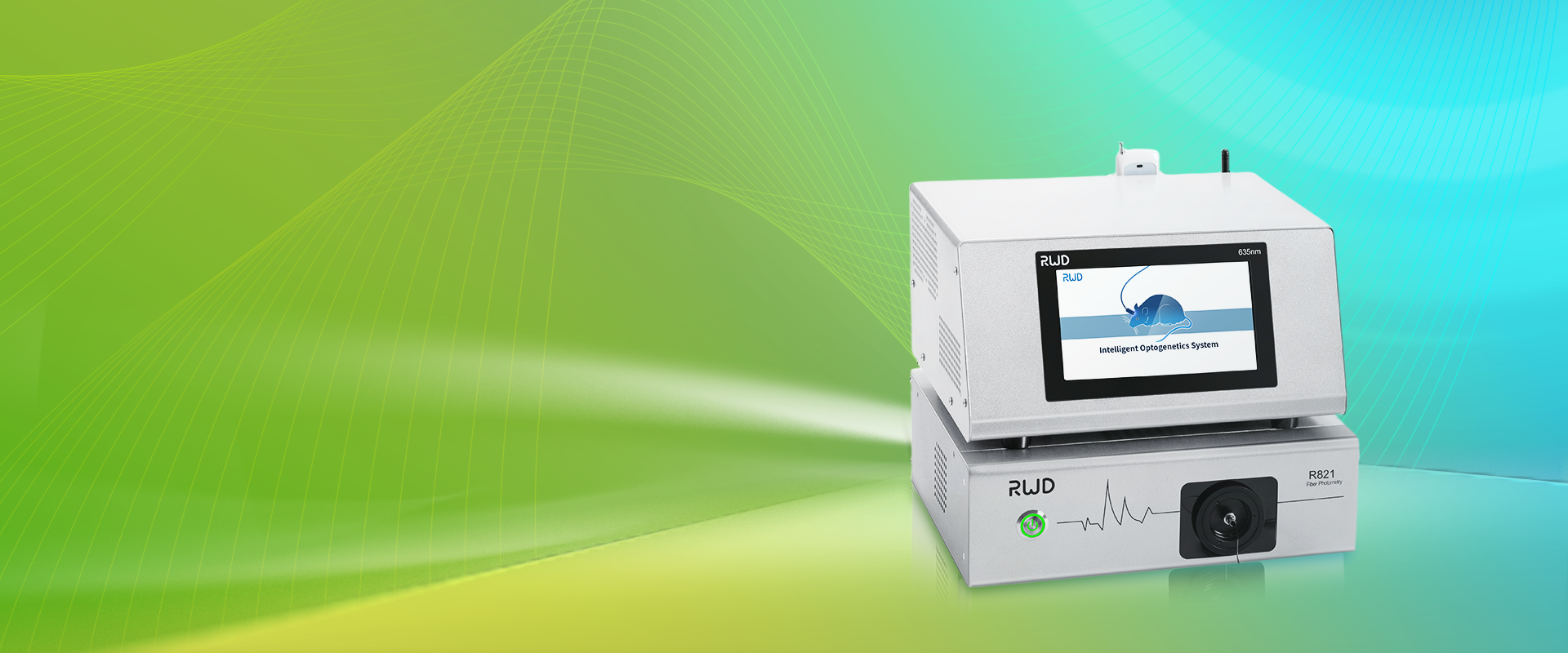
Hidden Flaws in Current In Vivo Imaging Systems
I want to be frank: the typical in vivo imaging system rarely fails for a single reason. Instead, several modest gaps stack up. First, many teams rely on default exposure or gain settings that suit one animal model but not another. That choice degrades the signal-to-noise ratio and reduces reliable quantitation. Second, environmental control (temperature, light leakage) is often treated as a “nice to have.” I’ve seen bioluminescence drift by 20% during a run because a warming lamp was left on — frustrating, yes, and avoidable.
Why does this fail?
Technical causes are simple. Fluorescence microscopy and photon flux both need consistent calibration. If you skip routine calibration or if your power converters—yes, the small PSU modules—sag slightly, the camera baseline shifts. Edge computing nodes used for real-time processing can help, but only if their clocks sync with acquisition hardware. Look, it’s simpler than you think: align the clocks, standardize gain, and log the room conditions. I often recommend a brief pre-run checklist. We add a quick phantom image and check the readout; if numbers swing, we pause and fix. This saves so much time later — funny how that works, right?
Principles for Next-Gen Approaches
When I think about the future, I focus on principles that matter more than gadgets. A smart in vivo imaging system blends stable hardware with simple software guards. For example, adaptive exposure that reads a control ROI and adjusts on the fly reduces overexposure of hot spots. Adding small telemetry — simple logs of temperature and power — lets you trace errors back to a cause. That is not flashy, but it is effective.
What’s Next
Practically, I advise teams to pilot a layered approach. First, tighten your baseline: regular calibration with phantoms, and track photon flux over time. Next, add lightweight QC scripts that flag sudden drops in signal-to-noise ratio. Finally, connect metadata: animal models, dose timing, and pharmacokinetics notes should ride with every image file. This lets you filter out false positives fast — and yes, it feels like breathing easier when your data behave. — and yes, I checked that this reduces re-runs by a noticeable margin.
Advice: How to Choose and Evaluate Solutions
I’ll leave you with three concrete metrics I use when I evaluate systems. First, stability: does the system hold a steady baseline over 24–72 hours? I look for <10% drift. Second, traceability: can you attach per-acquisition metadata (time, animal ID, temperature)? If not, it’s a red flag. Third, responsiveness: does the system adapt to changes in photon flux or high-intensity spots without manual rework? A positive here cuts rework by half in my experience. Use these metrics as your quick checklist — they work in most labs, small or large.
I’ve walked through what breaks, why it breaks, and what I’d change first. I share this from hands-on runs, not just theory, because I care about making your data honest and useful. If you want a sensible place to start, check practical toolsets and components from BPLabLine. We can be precise without being needlessly complex. I mean it — your next run can be better with small changes.